
The Loss Curve Was Fine
What a 4,096-expert router collapse taught me to measure
The loss curve was fine. That was the problem.
The legacy Super-4096 stress test, recorded as run_1768063844_579017 with 4096 routed experts and top-7 routing, kept improving on validation loss while its logged router snapshots concentrated brutally. In several layers, one expert appeared in nearly every token's selected set. Mean load imbalance climbed into the thousands of percent. At the reported endpoint, the worst logged layer had the entropy-equivalent support of roughly nine experts out of 4096.
I had been watching loss as if it were also a capacity-utilization metric. It had never agreed to that job.
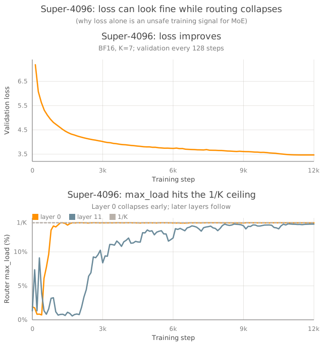
K saturation signature near 1/K.This is not the corrected Super-4096 run analyzed in 0006. It is an older, separate receipt surface. The figure's layer-order story belongs to that legacy run and should not be carried into the corrected one.
That run changed the questions I ask of a checkpoint. Is the fixed validation text compressing better? Did capability move beyond that text? Is the router still distributing traffic across the sparse capacity named in the config? Bits per byte, CORE, and the routing distribution answer those separately. When they disagree, the disagreement is usually the experiment, not dashboard clutter.
Compression needs the denominator back
Token-level cross-entropy is native to training and treacherous across tokenizers. Split the same byte sequence into different pieces and nats per token changes even when the underlying text does not.
Bits per byte puts the denominator back in the source. For a validation slice with mean loss L in nats per evaluated token,
On identical decoded bytes and an identical evaluation mask, bpb gives me a tokenizer-normalized comparison. “Normalized” is doing less work than people sometimes ask of it: change the text, byte accounting, normalization, mask, or tokenizer-dependent likelihood and the comparison changes too. It is not a universal unit smuggled out of thermodynamics.
The current trainer makes one further detail explicit. When valid/bpb is enabled, it uses a dedicated EOS-excluding loss and byte accumulator. Unless the masks happen to match, the canonical value cannot be reconstructed from valid/loss, valid/tokens, and valid/bytes after the fact. Existing miniseries runs therefore treat the logged valid/bpb as source of truth. The public contract would be cleaner still if it also exposed the bpb-specific loss sum.
This is the smooth curve I use for progress. It tells me whether a fixed validation stream is being compressed better. It says nothing by itself about what the model can do with that compression.
Capability arrives with wider error bars
For a broader read I use CORE, a suite of 22 heterogeneous multiple-choice, schema, and language-modeling tasks. Each task is centered against the random baseline supplied by the evaluation bundle. If accuracy is a and the baseline is b,
That prevents 50% on a binary task from pretending to be the same achievement as 50% on a four-way task. It does not make the tasks commensurate by decree. CORE is still an average over different behaviors, datasets, and sample counts, so I want the task vector whenever the aggregate moves.
It is also much noisier than bpb. On one miniseries slice, resampling the 22 task scores gives the following historical values. The exact task vectors and bootstrap outputs live in the external JSON artifacts named by the receipt; they are not bundled with this site.
| Checkpoint | CORE | Task-resampling 95% percentile interval |
|---|---|---|
step 863 | -0.0138 | [-0.081, 0.031] |
step 2156 | +0.0039 | [-0.071, 0.053] |
step 4312 | +0.0237 | [-0.025, 0.059] |
step 8624 | +0.0649 | [+0.024, +0.112] |
delta 863 → 8624 | +0.0787 | [+0.031, +0.137] |
The delta row resamples matched task positions together. Under that calculation the long-span improvement stays positive; the smaller intermediate movements do not separate cleanly. These are fixed, heterogeneous, correlated tasks, so the intervals describe sensitivity to suite composition—not a population confidence interval, and certainly not training-seed variance wearing a lab coat. They omit item-level uncertainty and repeated-run variance as well.
An evaluator failure must also remain distinguishable from a model miss. Expert-parallel evaluation takes a deliberately conservative path: rank 0 broadcasts an example index, every rank evaluates the same prompt, and rank 0 accumulates correctness. The current runner still catches rank-local exceptions as wrong answers without first establishing distributed error consensus. Those failures should invalidate the score; quietly lowering it is not robustness.
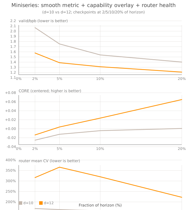
bpb moves smoothly; CORE arrives with wide task-level uncertainty; router health asks whether either curve came from the sparse system we intended to train.The router is not a warning light
It emits a distribution. Every scalar health metric is a projection of that distribution, which means every one of them is capable of lying by omission.
Let p_e be expert e's share of routed assignments in one layer for one logged global batch.
| Statistic | What it sees | What it can miss |
|---|---|---|
CV = std(load) / mean(load) | overall dispersion | whether imbalance is one hot expert or a long tail |
H = -Σ p_e log p_e | spread of assignment mass | which particular experts are hot or dead |
E_eff = exp(H) | entropy-equivalent support in expert-count units | the shape inside that support |
max_load = max(p_e) | the hottest expert | broad degradation outside the maximum |
| dead experts | zero assignments in that batch | whether zero load persists across batches |
Raw entropy is not comparable across expert counts because its maximum is log(E). I read both
This is exactly where the legacy Super-4096 dashboard tried to flatter me. Its externally recorded mean entropy, 4.15 nats, was numerically higher than the healthy MoE-64 value of 3.91. The pools were radically different sizes. Normalized, the values are about 0.50 for E=4096 and 0.94 for E=64; the impressive raw number represented a much smaller fraction of available support.
CV needs a regime too. If T tokens independently choose K distinct experts uniformly, expected rows per expert are μ = TK/E, and the assignment-count floor is
Batch size, E, K, and the particular logged batch all change what “large” means. A zero-load expert in one sparse snapshot is not permanently dead; proving persistence requires looking across batches.
max_load has one especially useful top-K signature. With distinct, unweighted selections and no dropped routes, an expert can appear at most once in each token's selected set. An expert selected for nearly every token therefore receives about 1/K of all assignments. That is a load statistic, not gate-weight importance. A layer pinned near 1/K has acquired a nearly universal expert for that batch.
Uniform routing is not the objective. Specialization should create structure. These measurements are canaries for support narrowing, not an invitation to flatten every expert into the same job (we already know how to build a dense model).
Three curves, one argument
The receipt's MoE-64 and legacy Super-4096 runs make the contrast visible, but they are not a controlled ablation: E, K, horizon, and schedule all differ. The exact comparison values below come from the external router-health artifact named in the receipt rather than a JSON payload shipped with the site.
| Metric | MoE-64 BF16 | Super-4096 |
|---|---|---|
| final validation loss | 3.43 | 3.47 |
| mean CV | 87% | 1733% |
mean H / log(E) | ~0.94 | ~0.50 |
worst-layer E_eff | ~44 / 64 | ~9 / 4096 |
The losses look similar. The assignment distributions do not. In practice I start with router_agg/mean_cv, router_agg/min_entropy, and per-layer max_load, then inspect the layers rather than letting an aggregate invent a topology. In the receipt's MoE-64 run, layer 0 approaches 1/K while the others remain broad. In the older Super-4096 surface, multiple layers pin near it on different schedules. One hot layer and depth-wide narrowing are different failures even when a single “router health” badge would color them the same.
Implementation details and exported figures are mapped in nmoe/repro/0002.receipts.json; its three measurement JSONs are external and not bundled with the site.
I still look at loss first. I just no longer let it testify for the rest of the system. Before I call a checkpoint better, I want the compression denominator, the task vector behind CORE, and the routing distribution that produced the sparse computation. One scalar can be perfectly correct and still be the wrong witness.