
The Experiment Had Two Model Sizes
A literal #420 transfer made the denominator part of the result
I copied the denominator along with the method. That was the mistake.
In nanochat discussion #420, Andrej Karpathy described a dense miniseries organized around one architecture dial, depth, with the rest of the family derived from it. The training horizon followed the ratio of tokens D to parameters N; for nanochat's small dense models, the fitted ratio landed near D/N = 8. I was attracted less to eight than to the discipline. Pick one dial. Derive the family. Make the cheap runs earn the expensive one.
I borrowed that grammar for nmoe. It was never a reproduction. The architecture, optimizer, and data path were different, but I wanted the same clean feeling of one knob controlling a family. At 20% of each model's separate D/N = 8 horizon, the first sparse slice looked obligingly good:
| Run | Depth | Routed experts | Tokens seen | valid bpb | centered CORE |
|---|---|---|---|---|---|
d10 | 10 | 64 | 759M | 1.40 | +0.001 |
d12 | 12 | 256 | 4.5B | 1.21 | +0.065 |
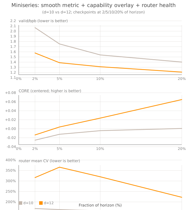
d12 had lower bpb and higher CORE. It had also seen almost six times as many tokens. I could make the plot confess to whichever story I preferred: depth helped, more experts helped, or more data helped. Three candidate causes in, zero isolated causes out. (The plot remained very handsome, which did not improve matters.)
The slash was hiding a second model
The transfer broke at a place dense scaling lets you ignore. Under the accounting convention here, a dense model has one parameter count because its total and active parameters are equal. An MoE stores every routed expert while each token selects only K of E in a sparse layer. Its size depends on whether I mean the stored model or the model traversed by one token.
nmoe therefore keeps both counts. P_total includes every trainable weight. P_active includes the non-routed path, every router, the selected fraction K/E of routed expert matrices, and the always-on shared experts. The corresponding data ratios are
The three models from 0003 were designed with nearly the same active FFN width per token, but radically different stored capacity:
| Model | Global P_total | Global P_active | P_total / P_active | Planned D/P_total | Planned D/P_active |
|---|---|---|---|---|---|
| Dense | 190.5M | 190.5M | 1.000 | 26.24 | 26.24 |
| MoE-64 | 755.5M | 191.1M | 3.954 | 6.62 | 26.17 |
| MoE-256 | 2.836B | 192.9M | 14.705 | 1.76 | 25.92 |
The last two columns use the planned 9536-step ceiling of 4,999,610,368 tokens. At that ceiling, 0003 was almost active-normalized. Its reported BF16 endpoints were not: the jobs stopped when they crossed the loss target, leaving realized tokens per active parameter of 22.89, 15.80, and 13.22 for dense, MoE-64, and MoE-256.
That distinction cost me another clean sentence. The 0003 configuration ceiling nearly matched active exposure; the observed stopping points did not. They also landed in different WSD phases, and the routed expert matrices used AdamW (0.9, 0.99) while non-routed groups used (0.9, 0.95). It was a threshold-crossing speedrun, not an equal-exposure ablation.
(The counts in the table are offline global reconstructions from the configs. The distributed helper sees rank-local expert tensors before global expert metadata is applied, so its output needs aggregation before I can use it as a global runtime count.)
I followed the other denominator
Keeping the dense speedrun's planned ratio,
gives full total-parameter horizons of 37,813 steps for MoE-64 and 141,963 for MoE-256 under the runner's floor rule. I have a provisional endpoint record at 20% of each sparse horizon:
| Endpoint record | Steps | Tokens seen | D/P_total | valid loss | CORE |
|---|---|---|---|---|---|
| MoE-64 | 7,563 | 3.965B | 5.24819 | 3.2625 | 0.051871 |
| MoE-256 | 28,393 | 14.886B | 5.24809 | 2.8554 | 0.145743 |
At those recorded endpoints, MoE-256 has the lower loss and higher CORE. It also received 3.754× as many tokens. That is not an accidental blemish on the comparison; it is the total-parameter contract doing exactly what it says. The model that stores more parameters gets proportionally more training. The result is not token-, FLOP-, or wall-clock-matched, and it does not isolate stored capacity as the cause of the difference.
I once called these endpoints closure. They are not. The bundle does not contain the resolved stage configs, run identities, logs, metric artifacts, or evaluation coverage, and it has no dense loss or CORE near the comparable step 1907. I am keeping the numbers because they are a useful endpoint record. I am not asking them to impersonate a qualified dense–sparse result.
The second denominator did not make the comparison cleaner. It made the missing controls impossible to ignore.
There is no innocent denominator
The comparison I still owe is a repeated-seed BF16 matrix over all three models at fixed fractions of both contracts, with data order, optimizer groups, schedule, validation, and CORE coverage held constant. It should report tokens, estimated FLOPs, training-loop time, memory, loss, and CORE together, because no denominator makes those costs equivalent by administrative decree.
Until that matrix exists, “fair” is too blunt a word. Active normalization budgets tokens against nominal per-token parameter mass. Total normalization budgets them against stored capacity and deliberately spends more training on models that store more. A compute budget, a memory budget, and a wall-clock budget ask different questions again and can favor different winners.
The first plot was not wasted. It taught me that D/N stops naming one experiment when N can describe either the stored model or the path a token actually takes. Dense scaling lets the slash look like arithmetic. In an MoE, the slash is part of the hypothesis.
Evidence: 0004 receipt · 0003 receipt. The d10/d12 slice is backed by the artifact paths recorded in 0004; the totalDN20 values remain a provisional endpoint record pending the missing configs and metrics.