One Boundary, Two Crossings

The first useful result from Super-4096 was not that the router had collapsed. It was that I could no longer say what collapse meant without lying by omission.

Loss kept falling while the routed layers used a steadily narrower part of their nominal expert capacity. That could mean the router had found an efficient specialization. It could mean the data had become repetitive. It could mean the experts were redundant, the backbone was steering every token into the same neighborhood, or the model was quietly destroying structure we would need later. A load histogram cannot distinguish those stories. Calling all of them collapse gives the uncertainty a dramatic name and then pretends the work is done.

I wanted a state variable with enough structure to ask the real question: what did pretraining build inside a sparse model, and did post-training preserve it?

The object we propose is the MoE Atlas. The paper makes one deliberately strong bet around it. Fix an operational Atlas contract before training: the probes, protected layers, measurements, tolerances, and target task criterion. A pretrained checkpoint becomes handoff-ready when it reaches the target while crossing into the acceptable region. A later checkpoint exhibits geometric forgetting when adaptation carries it out again.

Same boundary, opposite direction.

That symmetry is a definition. The claim that one such boundary can predict both continuation quality at handoff and retained capability after adaptation remains a hypothesis. We have the mathematical object, exact definitions of the receipts it would require, and partial trajectories in which objective progress separates from occupancy or routed-proxy recovery. We do not yet have the experiment that calibrates the boundary and watches capability cross it. The distinction is the whole paper.

The formal treatment is in The MoE Atlas. This is the argument that led us there.

A routed layer is not a bag of experts

Take the residual state immediately before a routed MoE layer. RMSNorm writes it as

At $\epsilon=0$, every nonzero ray lands on a sphere. At finite $\epsilon$ (the version models actually run), the image also retains a radial coordinate. More precisely, nonzero residual space factors into an angular direction $\omega=x/\lVert x\rVert$ and a radial fiber $a_\epsilon\in(0,\sqrt d)$. RMSNorm preserves the direction exactly.

This sounds like mathematical housekeeping until the router arrives. For a bias-free linear router, every score scales by the same positive radial factor, so top-$k$ membership depends only on $\omega$. The angular space is therefore cut into cells: inside a cell, the same exact set of experts is active; at its boundary, one expert can displace another.

The expert domains are a different object. With top-$k$ routing, every regular state belongs to $k$ expert domains at once. These domains overlap, and each expert supplies a local realization and a local output field on the portion it sees. The router cells say which set is selected. The overlapping expert cover says which local maps coexist. The routed layer glues their weighted fields together.

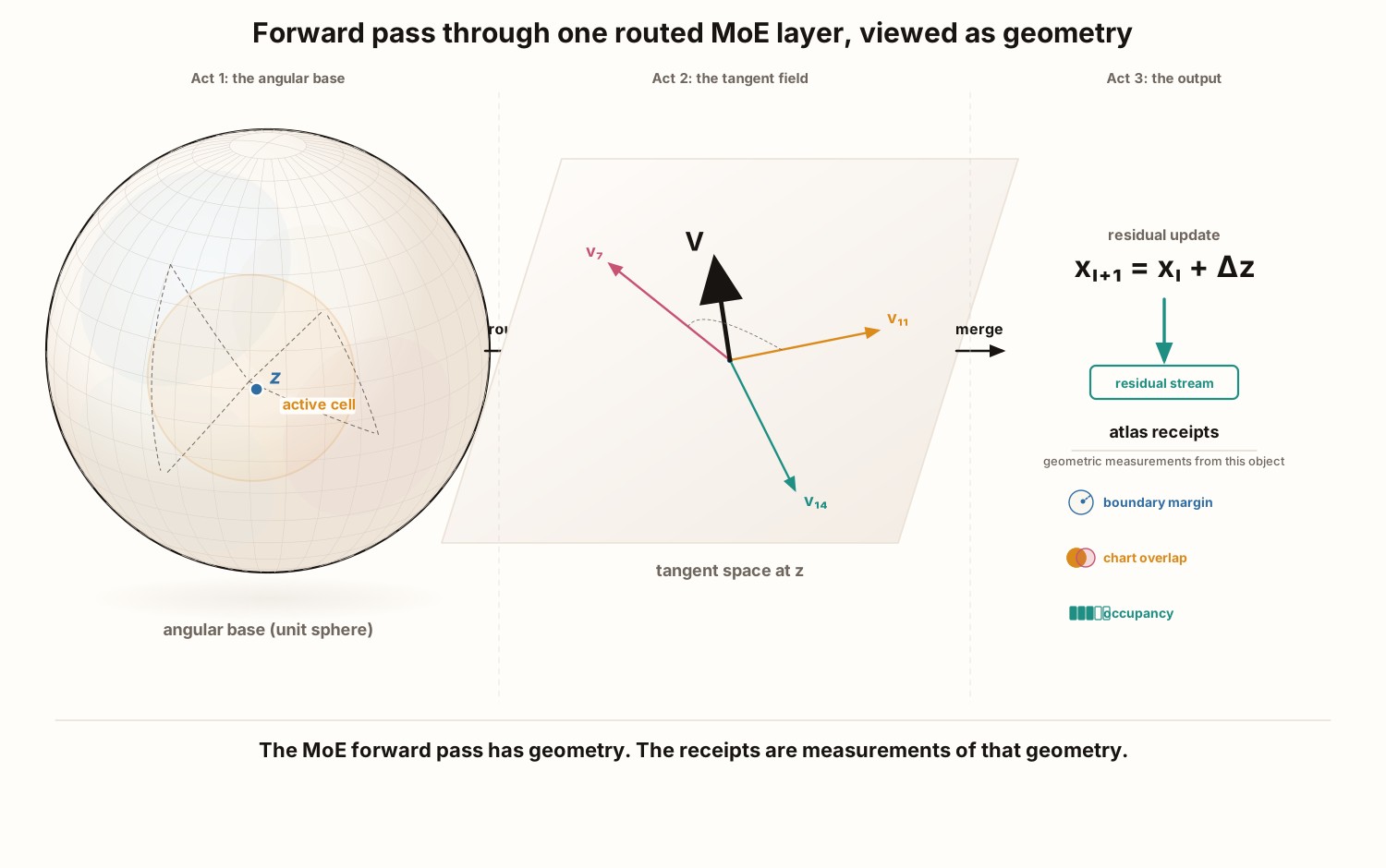
The word atlas is not there to make a tensor sound continental. It names the conditions under which those expert-local views really do behave like compatible local realizations of a shared state manifold.

Our first version demanded full column rank from every expert projection in the ambient hidden space. That was clean, powerful, and too strong for the fine-grained MoEs we actually care about, where expert width can be smaller than model width. The revised theorem asks for the rank that matters: if the states visiting a protected layer lie on an intrinsic $m$-dimensional manifold, each active expert map needs rank $m$ only on the tangent directions of that visited manifold. The ambient model can be huge. The expert has to resolve the directions the data actually uses.

For a linear router, the cells become unusually concrete. If $S$ is the active set and $b_e$ is expert $e$'s effective router normal, then

Every nonempty cell is a spherical slice of a strict polyhedral cone. It is contractible, and the exact geodesic distance from a state to the nearest exit is

The ordinary top-$k$ score gap gives a computable lower bound on this radius. A router margin is therefore not merely “confidence.” Once normalized by the competing router directions, it certifies how far a state can move before its active set must change.

That does not make a large margin automatically good. A model can be very far from a boundary because it has retreated into a tiny, impoverished part of the space. The geometry has to travel with occupancy.

What happens at the seam

Smooth pictures of neural networks tend to become coy exactly where routing becomes interesting. Hard top-$k$ is piecewise smooth. When a path crosses a generic one-swap boundary, one expert leaves and another enters. Under the paper's trace and weight-normalization assumptions, the jump in the routed field is the common boundary weight multiplied by the difference between the entering and departing expert fields.

That gives a local quantity with a physical interpretation: if adjacent experts produce compatible visible fields, the handoff is gentle; if they disagree, the composite field tears at the seam. Two experts can be close in parameter space and never be asked to substitute for one another. Another pair can look unrelated in a global similarity matrix yet share a dangerous routing boundary. Adjacency comes before similarity.

The revised paper pushes this past the polite one-boundary cartoon. Under finite-face and regularity assumptions, the hard-routed field is a bounded-variation field. Its singular variation is precisely the integral of these swap-boundary incompatibilities; there is no mysterious extra Cantor term hiding between cells. A centered perturbation bound then separates two ways the routed field can move: the router can redistribute weight across a set of expert fields, and the fields themselves can change. The router term scales with total-variation drift times the diameter of the affected fields, which makes the bound invariant to a shared translation of every expert output.

This is the level at which “the router changed” becomes a diagnosis instead of a mood.

The Atlas has a body and a weather system

The most important distinction in the paper is also the easiest to miss.

Under fixed routing semantics, the layer's gain, router, expert maps, cells, and participation domains define a structural Atlas. Freeze that surface and the structural object stays fixed.

But a running model also supplies a distribution of states that visits the Atlas. The backbone transports tokens into different coordinates; the data changes which regions are occupied; co-active neighborhoods appear and disappear. Pair the structural object with that transported probe or data measure and you get the operational Atlas state.

Freezing a road network does not freeze traffic.

This matters because the training intervention we kept describing as “frozen experts” did exactly what the phrase promises and much less than people hear in it. In a 64-expert Moonlight trajectory, the routed experts, shared experts, router, and feed-forward normalization were frozen. Distillation loss improved from 5.2479 at step 100 to 4.7968 at step 200 and roughly 4.5 later. Meanwhile a fixed-canary State-2 routed-geometry proxy moved from +0.0828 at the seed to -0.0632 at step 2000 after a partial rebound. Separately, live training-batch telemetry put load CV near 140% at the seed and roughly 190% later; minimum per-layer entropy moved from about 3.0 to 2.2, zero-load expert-layer incidences from 42 into the 225–300 range, and mean active experts per layer from 62.4 to roughly 55.

The proxy is not the paper's canonical co-active expert-field compatibility, and this run does not establish capability loss. It establishes something both narrower and firmer: objective improvement can coexist with degraded routed occupancy and proxy geometry even when the routed weights themselves do not move. The surrounding network can change the realized sparse system by changing what it sends through it.

The run that made the dashboard indefensible

The clearest evidence comes from a different model and a less flattering training record.

We reconstructed every available snapshot from a 64-GPU, 256-expert, top-8 pretraining run: step 1 and every ten steps through 2000, across 58 routed layers. The run presented 524,288,000 tokens, but those presentations repeatedly wrapped one 25-million-token shard. There is no held-out trajectory, the shard's corpus recipe is missing, and these receipts contain occupancy rather than the canonical Atlas fields. This is a systems trajectory, not a clean model-quality study.

Within that boundary, the split is difficult to ignore. Loss fell from 36.7413 to 9.7961. Mean load CV rose from 369.29% to 527.44%. Minimum per-layer load entropy fell from 2.9032 to 2.2961 nats. Zero-load expert-layer incidences in the logged windows rose from 8,088 to 11,708, while the mean active experts per routed layer fell from 116.55 to 54.14.

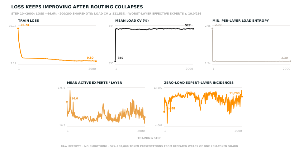
Loss did its job. It reported that the objective became cheaper on the repeatedly visited data. What it could not report was whether the model was approaching a good handoff state, memorizing a narrow shard, or sacrificing routed breadth that a later stage would need. Occupancy does not answer those questions either. The two signals simply refuse to stand in for one another.

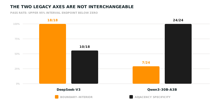
The same warning applies to geometry diagnostics themselves. On the heterogeneous checkpoint summaries we could audit, DeepSeek-V3 passed 18/18 layer checks on the legacy boundary-versus-interior axis but only 10/18 on the boundary-adjacent-versus-random axis. Qwen3-30B-A3B did almost the reverse: 7/24 and 24/24. Architecture, checkpoints, and data are not controlled across the two families, so this is not a model-family theorem. It is enough to kill the convenient assumption that nearby-sounding axes are interchangeable.

The 640-expert Legion lineage supplies scale context: real E640, top-16, world-64 execution, and a mixed expert bank. It does not supply a preservation result. We do not have a valid matched post-baseline pair or the full as-run freeze surface. It would be satisfying to put the largest model in the headline. It would also be false evidence, which is a rather high price for typography.

One boundary, if we can earn it

An operational Atlas contract fixes a probe family, protected layers, state coordinates, routing and field receipts, occupancy adjuncts, a baseline, tolerances, and a task-success criterion. Those choices define an acceptable region $\mathcal A$.

Then the lifecycle language becomes exact:

• readiness is an inward crossing into $\mathcal A$ while meeting the declared pretraining target;
• geometric forgetting is an outward crossing from $\mathcal A$ during later adaptation.

Neither word means universal readiness or human-visible forgetting. Both are relative to the registered probes and tolerances. A checkpoint can remain behaviorally competent after an outward crossing. Another can remain inside the region while failing the task for reasons the contract does not see. The wager is that a well-chosen boundary adds predictive information. A definition does not acquire causal powers by being typeset.

The observability result says when an output dashboard cannot settle the question. On a neighborhood of a checkpoint, let $B$ be a $C^1$, constant-rank map of output-only observables (losses, rewards, and differentiable benchmark surrogates) and let $L$ be a $C^1$ map of lifecycle receipts. Directions in the kernel of $dB$ leave the output dashboard unchanged to first order. If $dL$ still varies along those directions, the dashboard has an observability deficit:

This is not merely an existence proof that “metrics can miss things.” The rank counts the independent lifecycle directions invisible to the chosen dashboard, and any additional first-order receipt map that closes the gap must contribute at least $d_{\mathrm{miss}}$ scalar coordinates. If the lifecycle margin is locally constant on every output fiber, it factors through $B$ and the objection disappears. The theorem comes with its own escape hatch.

Hard routing makes those derivatives awkward at ties, so the paper also constructs a smooth bridge: an entropy-regularized top-$k$ inclusion vector on the hypersimplex. On finite probes and compact $C^1$ checkpoint families with a uniform positive routing gap, the smooth receipts are differentiable and converge uniformly to the hard ones. We can reason locally without quietly replacing the deployed router with a different model.

The experiment we owe

The current artifacts justify building the measuring instrument. They do not validate it.

The decisive study is preregistered and prospective. Choose the protected layers and Atlas boundary before looking at outcomes. Produce continuation pairs matched on loss and ordinary benchmarks but separated across the proposed margin. Continue both through the same downstream recipe. Ask whether the inward crossing predicts better continuation, whether the outward crossing predicts retained-capability loss, and whether an Atlas-directed intervention helps at matched task success.

The hypothesis should die if those pairs behave the same, if ordinary occupancy and output telemetry explain everything the Atlas adds, if the tangent-rank assumptions fail on the visited states, or if interventions that preserve the declared region do not improve retention. It should also die if we keep moving the boundary after every run until the pictures look prophetic.

The field has plenty of dashboards that narrate the past. I am interested in a contract severe enough to make a decision before the answer is known.

Pretraining readiness and forgetting have usually been treated as different problems because one happens before handoff and the other after it. Sparse models suggest a more economical possibility: perhaps both are questions about whether the same routed object is inside or outside a region we were brave enough to declare in advance.

We now know how to name that object. The next job is to find out whether it deserves the authority.

Paper: The MoE Atlas. Public artifact receipt: 0007.