Noumena

The comforting story about confidence is that when it fails, the dial points too high. Our runs found something worse: the dial barely moved while the thing underneath it changed sides.

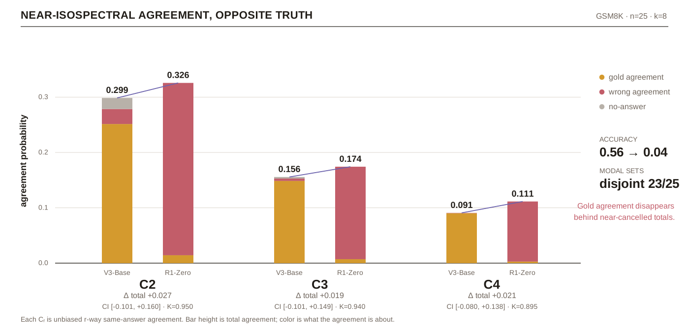
On a fixed slice of twenty-five GSM8K prompts, moving from DeepSeek-V3-Base to DeepSeek-R1-Zero took greedy accuracy from 0.56 to 0.04. The net was thirteen fewer correct prompts: fourteen regressed and one improved. The exact McNemar $p$ -value is 0.000977.

If that were the whole result it would be an ordinary, if unpleasant, benchmark regression. The strange part is what happened to agreement. We drew eight answers per prompt and measured the probability that two, three, or four independent draws return the same extracted answer. Across the slice, total agreement moved only from 0.2986 to 0.3257 at order two, 0.1557 to 0.1743 at order three, and 0.0909 to 0.1114 at order four. Every paired interval for those total changes crosses zero.

Inside it, agreement on the gold answer collapsed. The gold components of the order-two, -three, and -four spectrum fell from 0.2514, 0.1486, and 0.0903 to 0.0143, 0.0071, and 0.0029. Wrong-answer agreement rose from 0.0271, 0.0043, and 0.0006 to 0.3114, 0.1671, and 0.1086. All six semantic-component intervals exclude zero in the corresponding direction. The empirical modal-answer sets before and after post-training are disjoint on 23 of 25 prompts; their mean empirical total variation is 0.835.

We call this near-isospectral epistemic inversion. “Near” matters: the total spectrum was not proven identical. The inversion is that nearly the same low-order shape moved from agreement on gold answers to agreement on wrong ones.

Bar height is total agreement; color says what the agreement is about. The total deltas are unresolved, while gold and wrong components move decisively in opposite directions.

The full paper is Same Confidence, Opposite Truth: An Atlas of Hidden Answer Geometry. It began with a simple suspicion: confidence is not a property of one answer. It is a lossy view of a distribution we had declined to name.

Why DeepSeek-V3-Base and R1-Zero? When we ran the experiment, they were the best available pair for this question: a capable base checkpoint, a closely related post-trained model, and an R1-Zero regime strange enough to be worth cutting open. That regime is not a historical curiosity; we are still actively pursuing versions of it for both mathematical reasoning and code post-training.

If I restarted this particular measurement campaign today, I would probably use Kimi K2 Base and K2.7 Code as the contemporary pair and retain the DeepSeek comparison because the post-training regime remains scientifically live. GLM-5.2 would also be an obvious target, but without a matching base checkpoint it cannot support the before-and-after design this experiment needs.

The answer state is defined by a protocol

A language model does not carry a little Platonic probability distribution over “what it really believes.” It generates text under a protocol.

Fix the model $\theta$ , prompt $x$ , decoding policy $\pi$ , and a semantic extractor $g$ . Draw a completion

Y\sim P_{\theta,\pi}(\cdot\mid x),

then map it to an extracted answer $a=g(Y)$ . The induced distribution

p_{\theta,\pi,g,x}(a)=\Pr[g(Y)=a]

is the hidden answer state for that declared protocol. Its support includes an explicit no-answer outcome, $\bot$ , because failure to produce a parseable answer is not missing data. It is one of the things the model can repeatedly do.

Change the temperature, sampling rule, or extractor and you have changed the state being measured. That dependence is the honesty clause. Every confidence claim already depends on those choices; the protocol-defined state merely makes them visible.

The answer state lives on a labelled simplex. It can concentrate around the gold answer, settle into a repeatable wrong answer, fragment across incompatible answers, or collapse into $\bot$ . A scalar can say that mass became concentrated. It cannot, by itself, say where the mass went.

Self-consistency is a spectrometer before it is a vote

For an integer $r\ge2$ , define

C_r(p)=\sum_a p(a)^r.

This is exactly the probability that $r$ independent answers all agree. From a cloud of $k$ sampled answers, the all-subsets statistic

U_{r,k} = \binom{k}{r}^{-1} \sum_{|I|=r} \mathbf 1\{A_i=A_j\text{ for all }i,j\in I\}

is an unbiased estimator of $C_r$ . At $r=2$ , this is ordinary all-pairs self-consistency and $C_2=e^{-H_2}$ .

One sample cloud therefore measures a spectrum, not merely a winner.

With a known finite support bound $m$ , the power sums $C_1,\ldots,C_m$ recover the multiset of answer probabilities. In that precise sense, the agreement spectrum is complete for shape. But it is blind to a permutation of answer labels. A distribution with mass $(0.6,0.3,0.1)$ on (gold, wrong, none) has the same complete spectrum as one with those masses assigned (wrong, gold, none). Every order agrees because every order has forgotten the names.

The cure is not to abandon the spectrum. It is to put the labels back. For a prompt with gold answer $a^\star$ ,

C_r(p) = \underbrace{p(a^\star)^r}_{\text{gold}} + \underbrace{\sum_{a\notin\{a^\star,\bot\}}p(a)^r}_{\text{same wrong answer}} + \underbrace{p(\bot)^r}_{\text{no answer}}.

The power-sum spectrum is the shape chart. Gold, wrong, and no-answer occupancy say which outcomes carry that mass. Together they form the answer-state Atlas.

This “Atlas” is not the MoE Atlas from 0007. That one describes routed activation states, expert-local fields, and router cells. This one describes distributions over extracted semantic answers. There may eventually be a causal bridge between them. These experiments do not establish one, and sharing a good noun is not a proof.

Three ways to become more certain

The checkpoint comparisons move through the same answer space in three sharply different directions.

On GSM8K, the DeepSeek-V3 post-trained checkpoint produced what we would hope post-training means. Mean collision rose from 0.299 to 0.657, a paired change of +0.3586 with a 95% interval of [0.206, 0.504]. The increase came from repeated semantic answers while no-answer agreement fell. Observed greedy accuracy moved from 0.56 to 0.68, although that accuracy change alone is unresolved on this small slice ( $p=0.453$ ). This is beneficial consolidation: the answer cloud becomes more coherent in a useful semantic region.

DeepSeek-R1-Zero on the same GSM8K slice is the inversion from the opening. Its total spectrum barely changes, but agreement migrates from gold into wrong basins. The shape is familiar; the answers carrying it are not.

On the first fifty GPQA prompts, DeepSeek-R1 found a third path. Accuracy went from 0.26 to zero. Collision rose from 0.259 to 0.781, with a paired change of +0.5221 and interval [0.454, 0.587]. That looks like magnificent confidence until the extractor is allowed to testify: sampled no-answer mass rose from 0.345 to 0.810, and the greedy completion produced no extractable answer on 41 of 50 prompts. Repeated no-answer agreement increased while repeated semantic-answer agreement fell. The model had entered a no-answer attractor.

“Post-training sharpens the model” is true in roughly the way “the patient became quieter” is true. Direction is the clinical information.

Two wounds in the confidence surface

The checkpoint comparisons show that concentration needs labels. Controlled interventions reveal a deeper blind spot: even a fairly rich one-pass observer can remain fixed while the sampled answer cloud moves.

We recorded Shannon entropy, Rényi-2 entropy, two varentropies, maximum probability, margin, and the greedy answer at a prompt step. On GSM8K prompt 6 under V3-Base, every one of those values (and the correct greedy answer 260) was bit-identical before and after a final-layer intervention. Four sampled answers changed from

\{260,260,260,\bot\} \quad\longrightarrow\quad \{1.2,260,3,35\}.

Empirical answer-space $H_2$ moved from 0.470 to 1.386 and empirical total variation was 0.75. A second recorded run produced $\{1.2,260,260,35\}$ , again with the observer fixed.

On GPQA prompt 21, the greedy answer remained the same wrong choice, D, and the entire recorded observer again stayed bit-identical. This time even the empirical frequency multiset stayed fixed:

\{B,D,D,\bot\} \quad\longrightarrow\quad \{C,D,D,\bot\},

where C is gold. Both recorded runs reproduced the exchange. The quartet, $H_2=0.981$ , and every empirical power sum were identical. Labelled empirical total variation was 0.25.

Two observer-flat finite-cloud witnesses: a GSM8K answer cloud fragments while the observer and correct greedy answer stay fixed, and a GPQA wrong answer is replaced by the gold answer while both observer and agreement shape stay fixed. — Two nested blind spots. In the first row, the observer hides changing shape. In the second, even complete permutation-invariant shape hides changing semantic identity. 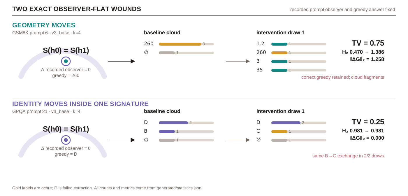Both are recorded `k=4` clouds.

These are exact statements about the recorded four-sample clouds. They are not powered certificates that the underlying population distributions differ. That boundary is particularly important because the broader perturbation record is mixed.

Under a strict prompt-by-prompt reconstruction, 18 nonbaseline conditions had enough local provenance to audit. Seven preserved every recorded observer coordinate exactly, and five of those had different semantically normalized empirical answer histograms. Two other conditions were incomplete. But a later targeted V3-only rerun found answer motion in 0 of 8 conditions, and four historical GSM8K movements vanished when 26 and 26.00 were normalized as the same number. The wounds exist in the retained samples. We have not established a stable perturbation mechanism or a prevalence rate.

Negative results are doing actual scientific work here. They stop an intriguing witness from quietly becoming a universal story.

Calibration cannot recover a coordinate it never saw

Let $\mathcal M_x$ be a local activation neighborhood. From a hidden state $h$ , the answer map $P(h)$ produces the protocol-defined answer distribution, while an observer $S(h)$ produces the recorded confidence statistics.

The clean question is whether the target answer quantity can be recovered from $S$ . Set-theoretically, the answer is exact: recovery is possible if and only if the target is constant on every fiber of $S$ (equivalently, if it factors through the observer). Measurable recovery needs the paper's additional measurability assumptions. If two states have the same $S$ value but target distance $d$ , any deterministic observer-only estimator has worst-case error at least $d/2$ on that pair; for a randomized observer-only estimator the same lower bound applies to worst-case expected error.

No amount of recalibration changes this. Calibration can repair a distorted coordinate. It cannot reconstruct variation that the projection erased.

The differential version counts the missing directions. Assume the observer and target spaces are finite-dimensional smooth manifolds and that $S$ and $f=T\circ P$ are smooth near $h$ ; then define

\ell_f(h) = \operatorname{rank}D(S,f)_h - \operatorname{rank}DS_h = \operatorname{rank}\!\left(Df_h\big|_{\ker DS_h}\right).

When $\ell_f(h)>0$ , there is a local direction that leaves the observer unchanged to first order while moving the answer target. In particular, if $\operatorname{rank}Df_h>\operatorname{rank}DS_h$ , such blindness is unavoidable.

This theorem does not say that every possible one-pass observer fails. A sufficiently informative observer may factor the target perfectly. It says we have to prove that relationship rather than infer it from a calibration curve.

What this result does—and does not—buy us

The checkpoint slices are small: 25 GSM8K prompts and 50 GPQA prompts, with eight samples each. They compare related checkpoints but do not causally identify a particular training update or dataset. The intervention cells were selected, correlated, and sampled only four times per prompt. The original generation launch command is missing: we can audit the retained receipts, but we cannot reproduce the exact launch bit for bit.

Within those limits, the central result is unusually clean. Total agreement at three orders can remain nearly unchanged while its gold and wrong components reverse. A one-pass confidence surface can collide on different empirical answer shapes. Even the complete permutation-invariant shape spectrum can collide on different semantic identities. And unconditional voting can turn a concentrated wrong mode into a more reliable wrong answer.

The next experiment should be prospective: preregister full task slices, increase the per-prompt sample count, repeat across multiple base-model families and pretraining checkpoints, and launch matched post-training branches. Then ask whether labelled answer geometry predicts which branches consolidate competence, which invert it, and when test-time compute helps rather than hardens the error.

Confidence, correctness, and legibility are different axes. Two answer states can share a silhouette and stand on opposite sides of truth; hidden answer geometry begins by refusing to mistake one for the other.

Paper: Same Confidence, Opposite Truth. Public artifact receipt: 0012.

Same Confidence, Opposite Truth